Executive Summary

When customers invest in a PV system, they often expect 25 to 30 years of energy production with minimal service and maintenance requirements. Depending on several factors, the system may or may not provide the financial performance that was originally expected. One factor that can lead to significant differences in the financial performance of a system is the design of the selected inverter.

Levelized cost of energy (LCOE) is a typical metric used to evaluate an energy system’s financial performance. Often when performing this calculation, a very detailed look at inverter replacement costs is not taken. However, there could be widely ranging differences in replacement or repair costs depending on the type of inverter chosen.

It behooves the PV industry to take a realistic look at lifetime costs and give customers up-front information regarding costs incurred after the system is commissioned. Unless the lifetime costs are explained clearly and truthfully to customers when the sale is made, a backlash could occur when they are surprised by inverter replacement costs. Since the industry has grown so rapidly in recent years, the majority of PV systems in the US are less than 5 years old, with typical standard inverter warranties being 5 to 10 years in length. Thus, the majority of inverters installed in the field are still under warranty and the industry has not needed to address large numbers of inverter replacements or repairs due to end of lifetime, though this will become commonplace as more and more PV systems age.

Fronius examined the possible costs associated with replacing or repairing inverters 15 to 20 years from now as the major differing factor in PV system cost of ownership. By estimating the total costs to maintain the PV system over its 25 to 30 year lifetime and comparing to the original purchase price, we can get an extended cost factor that shows how much more a system will cost over its lifetime based on the type of inverter chosen. For example, if the original system cost is $10,000 and the extended cost factor is 1.10, then the total cost of the system over its lifetime is $10,000 x 1.10 = $11,000. Based on the estimates given in the examples for three types of inverters, the following cost factors are derived:

While not all inverter manufacturers design their product with an eye towards field-serviceability, this is one area that could have a large impact on customer-borne costs when it comes to the inverter’s end of life. Designing and specifying field-serviceable inverters will minimize costs to bring the PV system back online at the end of inverter lifetime and allow the PV industry to enjoy a sustainable future.

Reliability and Service Life

Though the lifetime of PV systems can be 30 years or longer, power electronics often have lifetimes on the order of 15 years or less. Real-life data will be needed to get an accurate idea of product lifetime for all types of inverters. Fronius inverters are designed for a service life of 20 years. Mean time between failures (MTBF), which is sometimes misinterpreted to reflect lifetime, is simply a calculated reliability criterion that is only applicable during the normal useful life of the product. The typical “bathtub curve” of failure rate over time shows the three phases of a product’s life. 

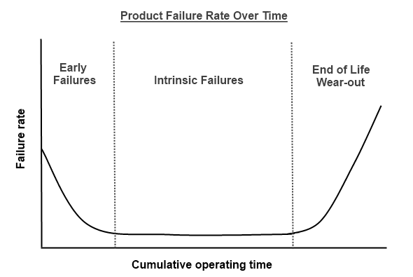
MTBF refers to the failure rate during the “intrinsic failures” period, and thus cannot be construed to give a picture of when wear-out could occur.

failure rate=  1/MTBF

A highly reliable product with high MTBF could reach wear-out in a relatively short time. Conversely, a product with low MTBF could reach wear-out after a much longer time.

In addition, it is important to note that an installation with many high-MTBF components could see more failures in its lifetime than one with a single lower-MTBF component. MTBF is expressed as the hours or years of total product operation before one failure occurs. For example, take a 7.5 kW PV system with 30 micro-inverters that have a calculated MTBF of 500 years. The calculated time to failure for this system would be

(500 yr)/(30 units)=16.7 yr/unit

This means that if the useful life of the inverters was beyond 16.7 years, there would be at least one failure within that time. Though the system would continue to operate at a lower capacity, the owner would generally prefer to have the system fixed and a service trip would be required, possibly under warranty. Comparably, a single string inverter used on this 7.5 kW system would only need an MTBF of 16.7 years to match the reliability of the micro-inverter system. A more realistic MTBF for string inverters is 100 to 200 years, indicating significantly higher reliability in terms of number of failures per system. Of course, MTBF expectations should be tempered with real-life data.

Code Updates

NFPA 70, the National Electrical Code, is updated and published every three years. Though many parts of the Code are well-established, new technology, research and improved safety measures can all prompt changes in any given revision cycle, even in something as time-tested as building wiring. In a newer area such as solar photovoltaic systems, much work is done every year to sort out all the changes necessary for this burgeoning technology. Section 690 was added to the Code in the 1984 edition. Throughout the last several revision cycles, some rather sweeping changes have been made to the requirements for PV installations. DC arc-fault circuit interruption, or instance, was introduced for building-mounted systems in 2011. A rapid shutdown system to control conductor voltage within ten feet of an array was introduced in 2014. As more and more PV systems are installed throughout the country, it is quite likely more attention will be paid to section 690 and result in more changes in requirements in future Code editions. Throughout a thirty-year life of a PV system, the opportunity for one or more significant Code changes becomes quite possible.

Changes in Technology

Being a growth industry, the technology landscape of photovoltaics and solar electronics is always changing. While transformer-based inverters dominated the technology landscape for a long time, transformerless designs are now becoming commonplace. Module-level electronics, whether retrofitted or module-integrated, are another recent area of advancement. As advances grow in this regard, significant changes to PV system design can result. As such, the products available on the market 15 years from now may very well look quite different from today. Field-proven advancements in technology can also help drive code changes, so module-level control being mandated in the future is a distinct possibility.

Serviceability

There are two ways in which field-serviceability of an inverter can affect system financial performance. First, system downtime can by minimized when failures occur. For either a failure during the warranty period or an end-of-life failure, the ability to troubleshoot and fix an inverter in one trip for the technician reduces the time that the system stays idle, waiting to be repaired. It is conceivable that if a data monitoring system detects an inverter failure, a technician could arrive on-site within 24 to 48 hours with a stock of replacement parts. The repair to the inverter can be done in minimal time in one trip and the system will resume full power production.

Compare this to a typical scenario where a technician makes a first trip to troubleshoot and determine the exact failure, then orders a replacement. String inverters are often replaced in whole, with wait times of one week typical for the replacement unit to arrive before the technician visits the site again. Altogether, this added wait time means about 450% more downtime compared to the field service case.

In the case of micro-inverters, let’s assume that all 30 inverters in a 7.5 kW system fail over a 5-year period near the end of their useful life. This would mean that 6 inverters fail per year or an average of one every two months. Let’s assume that a technician arrives with two replacement inverters a week after every second inverter failure. This would mean that half the system is down for about 67 days and the other half is down for 7 days. This means the whole system is down for an average of 37 days, amounting to 1850% more downtime than the field service case.

The second and most dramatic way in which field-serviceability affects financial performance is by reducing the total costs incurred when the inverter must be repaired or replaced at the end of life. These effects are demonstrated in the following examples.

Examples

Though it is impossible to know exactly what will happen in the future, some reasonable assumptions can be made in order to get a range of costs that could be expected over a 30-year timeframe. Fronius examined how the serviceability of the inverter affects long term costs in three different cases by assuming a 7.5 kW residential PV system and calculating the total cost of ownership (TCO) for each case. Since the up-front cost is the most visible to the end customer, TCO is compared to the initial system price to give a simple metric to compare the three cases – the extended system cost factor. The three cases examined are:

1)     A typical string inverter installation where the inverter must be replaced at the end of its service life

2)     A micro-inverter installation where the inverters must be replaced at the end of their service life

3)     A string inverter installation where the original inverter can be serviced with new parts

In order to derive the calculations, some assumptions had to be made. In all cases, it is assumed that the inverter reaches its end of life outside the warranty period but within the PV system lifetime, such that the inverter must be repaired or replaced at cost to the system owner in order to maintain energy output. This allows for a 15 to 20 year useful life of the power electronics. A $600 catch-all for other system service and maintenance is included.  The site is assumed to be a 50-mile, 1-hour drive (each way) for the company servicing the inverter, with a $3.50/gal fuel price and 15 miles/gal vehicle efficiency. Other assumptions specific to each case are denoted within the example. Technician labor is valued at $50.30 per hour.[1] Engineering labor is valued at $100 per hour. All values are in today’s dollars. For these examples, the “cost” of downtime is not factored in.

Example 1: Typical String Inverter

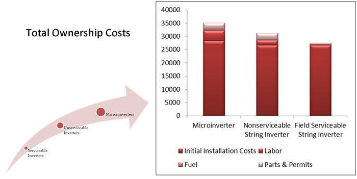
In this case, a single string inverter is used and it must be replaced with a new unit at the end of its service life, in the typical fashion that most residential PV systems are installed today. Once the inverter fails, a technician would visit the site to troubleshoot and determine what needs to be replaced or updated. Since the electrical system is being altered with new equipment, an electrical inspection must occur and the system be brought up to code, which also adds cost. As mentioned earlier, it is quite possible that module-level control of the system would be commonplace due to code changes and/or technical advancements. An engineer would need to select a replacement inverter and design other parts of the system. In addition, as this new inverter likely has some different output characteristics, the interconnection agreement with the utility must be updated. Two technicians return to install the new inverter as well as the module-level electronics on the roof. Twenty-four minutes are allocated to remove each module, add electronics and reinstall on the racking, based on NREL installation time estimates.[2] These costs as delineated in the table below account for a 19% higher TCO compared to the initial installation cost.

Example 2: Micro-inverters

For example 2, we take the case of a micro-inverter installation, assuming one inverter per 250W module, for a total of 30 inverters. We assume that once two micro-inverters fail (6.7% of the total system) they are then replaced with new ones at the same time to save on installation. Two technicians are required since they must get on the roof to replace the broken inverters, but they make only one site visit as it is assumed that monitoring alone can determine the need for inverter replacement, thus eliminating a troubleshooting trip. Though not necessarily the case, we assume that no inspection will be needed to replace the individual micro-inverters with new models. However, again the interconnection agreement must be updated, perhaps more than once as different models are added to the system. The costs delineated below show a 26% higher TCO compared to initial installation cost.

Example 3: Serviceable String Inverter

For example 3, a string inverter is used that can be repaired with replacement parts at the end of its service life. Once the inverter fails, a technician would visit the site to troubleshoot and determine what needs to be replaced. Since the electrical system is not being altered with new equipment, an electrical inspection is not needed. No engineering or updated interconnection agreement is needed. The technician repairs the inverter during the same trip with spare parts stocked on-hand. The costs delineated below shows just 5% higher TCO compared to initial installation cost.

Conclusions

By examining the differences in cost of service and downtime between three types of PV systems, we have demonstrated that the lowest TCO, and thus lowest LCOE, can be achieved by utilizing a field-serviceable string inverter. Fronius believes that the end of life costs associated with the replacement of inverters need to be fully accounted for and disclosed to the customer in order for the PV industry to maintain a professional, trusted image. Utilizing string inverters designed for field service will help reduce overall costs and thus move the industry forward.

[1] Ardani, K.; Barbose, G.; Margolis, R.; Wiser, R.; Feldman, D.; Ong, S. (2012). Benchmarking Non-Hardware Balance of System (Soft) Costs for U.S. Photovoltaic Systems Using a Data-Driven Analysis from PV Installer Survey Results. DOE/GO-10212-3834. Washington, DC: U.S. Department of Energy.

[2] Goodrich, A.; James, T.; Woodhouse, M. (2010). Residential, Commercial, and Utility-Scale Photovoltaic (PV) System Prices in the United States: Current Drivers and Cost-Reduction Opportunities. NREL/TP-6A20-53347. Golden, CO: National Renewable Energy Laboratory.

The content & opinions in this article are the author’s and do not necessarily represent the views of AltEnergyMag

Featured Product

QuickBOLT - QB RibRider: Flexible, Fast, and Secure Solar Mounting for Metal Roofs

The QB RibRider™ is an adjustable and easy-to-place mount for exposed fastener and trapezoidal ribbed roofs, combining versatility with robust construction. It features a 90/180 mounting combo with 75mm butyl pads on the base for superior weatherproofing. The RibRider is designed to fit most exposed fastener, trapezoidal, and ribbed metal roof profiles. This mount features stainless steel roof brackets and comes with four #14 x 1-1/4" hex washer self-drilling screws, ensuring a secure attachment to the roof.

More Products

Feature Your Product